


PEFT - Parameter Efficient Fine-Tuning: A Survey


This post is a joint work with Moshe Mishan (@datainsightsbymoshe)
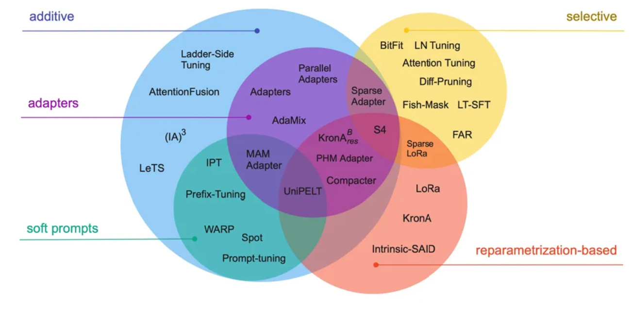
Large Language Models (LLMs) like GPT, Claude, and LLaMA have revolutionized natural language processing (NLP), powering applications from conversational AI to code generation. However, their immense size and computational demands present challenges when adapting them to specific tasks. Parameter-Efficient Fine-Tuning (PEFT) offers an elegant solution by enabling task-specific adaptation with minimal resource requirements. This blog explores the nuances of PEFT, the methods that make it possible, and the cutting-edge strategies for its application. This blog post will review the PEFT methods, organized by the three major families outlined in the survey paper "Parameter-Efficient Fine-Tuning for Large Models": Additive fine-tuning, Selective fine-tuning, and Reparameterized fine-tuning. We will focus on representative methods from each family, delving into their core mechanisms and mathematical formulations.
What is PEFT and Why is it Needed?
PEFT is a methodology for fine-tuning large models by adjusting only a subset of their parameters or incorporating lightweight structures into the model. The primary objectives are:
Efficiency: Reduce the computational cost and memory requirements of fine-tuning.
Scalability: Enable fine-tuning for tasks where full model training is impractical due to hardware or time constraints.
Reusability: Facilitate multi-tasking or domain-specific tuning without duplicating the full model.
Traditional fine-tuning adjusts all model parameters, requiring enormous computational resources and storage. PEFT sidesteps this challenge, focusing on efficiency without significant compromises on performance.
Main Challenges in Full Fine-Tuning LLMs
1. Resource Intensity
Compute: Updating billions(sometimes dozens or even hundred of billions) of model parameters requires substantial computational resources, including many powerful GPUs or TPUs and considerable training time. This limits accessibility and scalability. For instance, fine-tuning models like GPT-3 on even moderately sized datasets can be prohibitively expensive for many research labs and individual researchers.
Memory: LLMs with billions of parameters demand substantial memory for storing gradients, KV-cache and activations during training.
Storage: Fine-tuned models are typically the same size as the original pre-trained model, leading to significant storage requirements, especially when dealing with numerous fine-tuned versions for different tasks.
2. Overfitting
Fine-tuning all parameters on small task-specific datasets increases the risk of overfitting, reducing generalization performance.
3. Catastrophic Forgetting
Models fine-tuned on new tasks may lose performance on previously learned tasks, especially in multi-task or continual learning settings.
The Need for Parameter-Efficient Methods
PEFT addresses these challenges by limiting the number of trainable parameters, resulting in:
Reduced resource consumption during fine-tuning.
Faster experimentation cycles due to lower computational overhead.
Ease of storage with compact task-specific parameter updates instead of full model copies.
Resource Considerations in PEFT
Compute: PEFT minimizes backpropagation through the majority of the model, reducing compute requirements.
Memory: Memory usage is reduced as fewer parameters are updated and stored.
Storage: Task-specific adapters or weight deltas are orders of magnitude smaller than the full model, facilitating scalability.
Energy Efficiency: PEFT methods consume less power, aligning with sustainable AI goals.
PEFT Techniques
Additive PEFT
This family of Parameter-Efficient Fine-Tuning (PEFT) methods focuses on augmenting a pre-trained model by introducing new, trainable parameters, while the original model parameters remain frozen(not optimized during fine-tuning). The core idea is to inject task-specific knowledge through these newly added modules, often implemented as lightweight layers or vectors/matrices placed within the model's architecture. These added parameters are then optimized during the fine-tuning process, enabling the model to adapt to the target task without modifying the pre-trained knowledge encoded in the original weights. Techniques like Adapter modules and Prompt-Tuning fall under this category, demonstrating the effectiveness of targeted parameter addition for efficient fine-tuning. A key advantage of additive methods is their modularity, allowing for the easy addition or removal of task-specific modules without altering the base model, enabling multi-task learning and easier experimentation. Additionally, the original weights are kept unchanged, preserving the pre-trained model's general knowledge and avoiding catastrophic forgetting.
Adapters
Adapters are small, task-specific trainable modules into the pre-trained language model's architecture while keeping the original LLM weights frozen. These modules are typically inserted after the attention and feed-forward layers within each transformer block. A common structure for an adapter module involves a down-projection layer(linear), a non-linear activation function, and an up-projection layer. This bottleneck architecture forces the adapter to learn compressed representations of the task-specific information.
By only training the parameters within these newly introduced adapter modules, the number of trainable parameters is significantly reduced compared to full fine-tuning. The size of the adapter modules (specifically the bottleneck dimension) determines the number of additional parameters.
Structure: An adapter module is typically inserted after the attention mechanism and the feed-forward network within each transformer block. A common structure for an adapter is a bottleneck architecture:
Down-Projection Layer: Reduces the dimensionality of the input activation. The down-projection layer is a linear transformation:
where
h is the output of a transformer sub-layer (e.g., attention).
Non-linearity: An activation function applied to the down-projected representation, often ReLU:
\(h_{nonlin} = ReLU(h_{down})\)Up-Projection Layer: Projects the reduced-dimensional representation back to the original dimensionality:
\(h_{up} = W_{up}h_{nonlin} +b_{up}\ \text{where}\ \ W_{up} \in R^{d_{adapter}*d_{model}},\ b_{up}\in R^{d_{model}}\)Residual Connection: The output of the adapter is added to the original activation via a residual connection:
\(h_{adapter} = h + h_{up}\)Trainable Parameters: The weights and biases of the down-projection (W_down , b_down ) and up-projection (W_up , b_up ) layers within the adapter module are the only trainable parameters.
Insertion Point: If the output of a transformer sub-layer is F(x), the integration of the adapter can be represented as:
\(\text{Adapter}(F(x)) = F(x) + W_{\text{up}} \cdot \text{ReLU}(W_{\text{down}} F(x) + b_{\text{down}}) + b_{\text{up}} \)Benefits:
Minimal additional parameters.
Easy insertion and removal for multi-task applications.
Efficient scalability for low-resource or multilingual tasks.
Relevant Papers:
Prompt Tuning
Prompt tuning prepends a small, trainable continuous vector (the soft "prompt") to the input sequence. The parameters of the pre-trained LLM are frozen, and only the parameters of this prompt vector are learned during fine-tuning. The LLM then processes the input with this learned prompt, effectively guiding its behavior towards the desired task. The number of trainable parameters is simply the length of the prompt vector multiplied by its dimensionality, which is typically very small compared to the LLM's parameters.
Structure: A trainable embedding layer generates the soft prompt. Let the input sequence of the embedding vectors be:
\(E=[e_1,e_2,...,e_n] \ \text{where}\ e_i\in R^{d_{model}}\)Here i-th vector encodes the i-th sequence token . The soft prompt is a sequence of m trainable vectors:
\(P=[p_1,p_2,..., p_m]\ \text{where}\ p_i\in R^{d_{prompt}}, i=1, 2,...,m. \)Typically d_prompt=d_model.
Input to the LLM: The input to the language model becomes the concatenation of the soft prompt and the original input embeddings:
Trainable Parameters: The elements of the prompt embeddings p1...pm are the trainable parameters.
Benefits:
Involves relatively small trainable parameters (usually a few thousand).
Easy to implement.
Relevant Papers:
Selective PEFT
This family of PEFT methods takes a different approach by focusing on updating only a carefully selected subset of the pre-trained model's existing parameters. Instead of introducing new parameters, selective fine-tuning methods aim to pinpoint the most relevant parameters for a given task, leaving the rest frozen. This selection can be based on various criteria, such as layer-wise importance, attention head relevance, or specific activation patterns. By updating only the necessary parameters, these techniques significantly reduce the computational overhead and memory footprint associated with fine-tuning large language models. Methods like BitFit, where only the bias terms are trained, exemplify this parameter-efficient approach. The primary advantage of selective fine-tuning lies in its extreme parameter efficiency, often requiring the training of only a very small fraction of the model's total parameters. This makes it especially suitable for resource-constrained environments and when the fine-tuning dataset is relatively small, while still achieving reasonable performance.
BitFit
BitFit is an extremely simple selective fine-tuning method where only the bias terms of the network are trained. All the weight matrices remain frozen.
Structure: For a linear layer y=Wx+b only the bias vector b is updated during training. The weight matrix W remains frozen(= untrained) at its pre-trained values.
Trainable Parameters: Only the bias vectors of the linear layers and potentially the layer normalization layers are trainable.
Benefits:
It drastically reduces the number of trainable parameters, requiring far less memory and computation during fine-tuning compared to methods that update weight matrices. This makes it particularly suitable for very large models and resource-constrained settings.
By updating only biased terms, BitFit is less prone to overfitting, especially when fine-tuning on limited datasets. This encourages the model to rely more on the knowledge gained during pre-training.
Relevant Papers:
Reparameterized PEFT
Reparameterization methods tackle parameter efficiency by re-expressing the model parameter updates (not the weights themselves!) within the pre-trained model using a more compact representation. The core idea is that the full weight update matrix, especially for large models, can be approximated with lower-rank matrices or other parameterizations. During fine-tuning, these new parameterizations are optimized, and their effect is then applied to update the original model weights. This allows for an indirect manipulation of a large number of weights with a comparatively low number of training parameters. A prime example of this approach is Low-Rank Adaptation (LoRA), which uses trainable low-rank matrices to approximate the full weight update, demonstrating that effective adaptation can be achieved with only a fraction of the parameters modified. The key advantage of reparameterization techniques is their ability to approximate full model fine-tuning performance while using a significantly smaller set of parameters. They offer a good balance between performance and parameter efficiency, making them a very powerful and practical solution for fine-tuning large language models.
LoRA Family of Methods
The LoRA family of techniques represents a significant branch of PEFT, sharing the core principle of adapting pre-trained LLMs by injecting(adding) trainable low-rank matrices into the existing weight matrices. The foundational LoRA technique achieves parameter efficiency by approximating the weight updates during fine-tuning with these smaller, low-rank matrices, typically applied to the attention layers. This approach allows for effective adaptation while training only a small fraction of the total parameters. Building upon this core idea, subsequent methods within the LoRA family, such as QLoRA, GaLoRe, and DoRA, introduce further innovations, including quantization for memory efficiency, modifications to the gradient update process, and the incorporation of scaling factors, all while retaining the fundamental low-rank adaptation strategy to achieve efficient and performant LLM fine-tuning.
Low-Rank Adaptation (LoRA)
LoRA freezes the pre-trained weights of the LLM and injects trainable low-rank matrices into the attention blocks (specifically, into the weight matrices of the query, key, and value projections). For a weight matrix
LoRA introduces two smaller matrices:
During the fine-tuning only A and B are trained, and the update train matrix is given by W=W_0+AB. The key insight is that the updates to the weight matrices during adaptation often have a low intrinsic rank. The number of trainable parameters is determined by the rank r and the dimensions of the original weight matrices. Since r is much smaller than the original dimensions, the number of trainable parameters is significantly reduced.
Structure: As we mentioned earlier, for a given weight matrix W_0 in the pre-trained transformer, LoRA introduces two low-rank trainable matrices A and B.
Weights Update: The adapted weight matrix W is given by:
\(W=W_0+W=W_0+BA.\)
Linear Layer with LoRA: Consider a linear layer operation y = W_0x. With LoRA, this becomes:
\(y:=(W_0+BA)x =W_0x+BAx\)Trainable Parameters: The elements of the low-rank matrices A and B are the trainable parameters. The number of trainable parameters is: dr+kr= r(d+k).
Integration into Transformer: LoRA is typically applied to the weight matrices of the query W_q, key W_k and value W_v projections in the multi-head attention mechanism. For example, for the query projection:
\(Q=(W_{q,0} + B_qA_q)x\)where W_{q,0} are the frozen pre-trained query weights, and B_q and A_q are the trainable LoRA matrices.
Key Features:
Utilizes low-rank matrices to update model weights, which significantly reduces the number of trainable parameters.
Maintains the integrity of the original model by adding these low-rank updates to specific layers rather than modifying the entire model.
Advantages:
Offers a way to fine-tune LLMs with much less computational overhead, making it feasible for environments with limited resources.
Allows for quick adaptation to new tasks or domains without extensive retraining, enhancing model versatility and efficiency.
Relevant Papers:
QLoRA (Quantized LoRA)
QLoRA builds upon LoRA by introducing quantization techniques to further reduce memory footprint during fine-tuning. It freezes the pre-trained LLM after quantizing it to 4-bit precision (using a novel NormalFloat4 data type) and then trains LoRA adapters on top of these frozen, quantized weights. The NormalFloat4 quantization is specifically designed to minimize information loss during the quantization process. QLoRA also utilizes a technique called double quantization to further reduce memory usage of the quantization constants.
Structure:
4-bit NormalFloat Quantization: The pre-trained LLM weights are quantized to 4-bit NormalFloat (NF4). This involves mapping the original full-precision weights to a discretized set of values. Let Q(.) denote the quantization function. The quantized weight matrix W_{quant} is a quantized version of Q_0.
Freezing Quantized Weights: These 4-bit quantized weights are frozen during fine-tuning.
LoRA Adapters: LoRA adapters (low-rank matrices A and B) are introduced as in the original LoRA method, but they operate on top of the frozen quantized weights.
Weight Update: The effective weight matrix used during the forward pass is dequantized and combined with the LoRA update:
\(W_{effective}=D(W_{quant})+BA\)where D() is the quantization function that maps the 4-bit values back to higher precision.
Trainable Parameters: Only the elements of LoRA matrices A and B are trained in higher precision.
Double Quantization: QLoRA also employs double quantization to reduce the memory footprint of the quantization constants, further saving memory.
Key Features:
Incorporates 4-bit quantization for weights and gradients, drastically reducing memory usage.
Ensures minimal performance degradation by leveraging mixed-precision computations.
Advantages:
Enables fine-tuning of billion-parameter models on commodity GPUs, democratizing access to LLM fine-tuning.
Relevant Papers:
GaLoRe (Gradient Low-Rank Projection)
Instead of directly adding low-rank matrices to the weight matrices like LoRA, GaLoRe introduces trainable low-rank matrices to the gradient updates. During backpropagation, the gradients are projected onto a low-rank subspace defined by these trainable matrices. This allows for a more dynamic and nuanced adaptation of the model based on the actual gradient information. The number of trainable parameters is determined by the rank of the gradient projection matrices. Since this rank is typically much smaller than the dimensions of the weight matrices, the number of trainable parameters is significantly reduced.
Structure: During backpropagation, the gradient of the loss with respect to a weight matrix W_0 denoted as ∇_{w₀}L , is projected onto a low-rank subspace. This is achieved by introducing two trainable matrices
\(P\in R^{d\text{x}r} \ \text{and}\ Q\in R^{k\text{x}r},\ \text{where}\ r<< min(d,k)\ \text{and L is the loss function.}\)Gradient Update: The effective gradient update W is formed by the outer product of the transformed gradients:
\(W=({\nabla_{w_0}} LP)Q^T\)
where the multiplication is performed such that the dimensions align correctly.
Weight Update: The weight update rule becomes(for plain SGD):
\(W_{t+1}=W_t-ηΔW=W_t−η\nabla_{w_0}L PQ^T\)
where η is the learning rate. For ADAM, RMSProp and other advanced optimization methods the computation can be easily adjusted.
Trainable Parameters: The elements of the matrices P and Q are trainable parameters.
Integration: This method modifies the backpropagation step to incorporate the low-rank projection of the gradients.
Advantages:
Facilitates seamless adaptation across modalities, enhancing performance in multi-modal settings.
By operating on the gradients, GaLoRe can potentially achieve more effective adaptation by focusing on the directions of change.
Adapts the model based on the actual gradients, allowing for more fine-grained control over the learning process.
Relevant Papers:
Optimization Strategies for PEFT
While PEFT methods already significantly reduce the trainable parameters, further optimization techniques can be employed to enhance efficiency, reduce model size, and potentially improve inference speed. Pruning and Quantization(as in QLoRa and GaLoRe) are two prominent strategies that can be effectively combined with PEFT to achieve these goals.
Pruning Strategies for PEFT
Pruning techniques aim to identify and eliminate less important weights or connections within the neural network, thereby reducing the active parameter set during fine-tuning and inference. When applied in conjunction with PEFT methods, pruning can further minimize the overhead introduced by the additional trainable parameters or optimize the already parameter-efficient model. Pruning strategies can be broadly categorized as follows:
Structured Pruning: Structured pruning removes entire structural units of the network, such as rows, columns, filters, channels, or even entire layers. In the context of PEFT, structured pruning can be applied to:
Adapter Modules: Removing entire adapter layers or specific neurons within adapter modules to reduce the number of adapter parameters and potentially inference latency introduced by adapters.
LoRA Matrices: Eliminating entire rows or columns from the low-rank matrices (A and B in LoRA) used for adaptation. This reduces the rank and thus the number of trainable parameters, potentially simplifying the adaptation process without significant performance degradation.
Benefits: Structured pruning often leads to hardware-friendly sparsity, as it removes contiguous blocks of weights, which can be efficiently exploited by optimized libraries and hardware accelerators.
Unstructured Pruning: Unstructured pruning, in contrast, removes individual weights based on certain importance criteria. These criteria can be magnitude-based (removing weights with the smallest absolute values) or gradient-based (removing weights with the smallest gradient magnitudes or contributions to the loss). In PEFT, unstructured pruning can be applied to:
Fine-tuned Parameters: Directly prune the weights of the adapter modules or the LoRA matrices based on their importance.
Benefits: Unstructured pruning can achieve higher sparsity levels compared to structured pruning, potentially leading to greater model size reduction and faster inference on specialized hardware. However, it often results in irregular sparsity patterns, which might be less efficiently exploited on general-purpose hardware.
Dynamic Pruning: Dynamic pruning strategies adjust the pruning mask during the training process itself. Instead of applying pruning only once before or after training, dynamic pruning iteratively evaluates the importance of weights and updates the pruning mask in response to the evolving task requirements and the current state of the model. In the context of PEFT, dynamic pruning could be used to:
Adaptive Adapter Pruning: Gradually prune adapter parameters during fine-tuning, allowing the model to learn which parts of the adapters are most crucial for the specific task.
LoRA Rank Adaptation: Dynamically adjust the rank r in LoRA based on performance metrics during training, effectively pruning or expanding the low-rank subspace as needed.
Benefits: Dynamic pruning can lead to more robust and task-specific pruning, potentially achieving a better trade-off between model size and performance compared to static pruning methods.
Quantization Strategies for PEFT
Quantization techniques reduce the numerical precision of the model's parameters and/or activations, aiming to balance efficiency gains (smaller model size, faster computation, lower memory bandwidth) with acceptable levels of accuracy. When combined with PEFT, quantization can further optimize the already efficient fine-tuned models for deployment and resource-constrained environments. Common quantization strategies include:
Post-Training Quantization (PTQ): Post-Training Quantization is the simplest form of quantization, where the pre-trained (or fine-tuned) model weights are quantized after the training process is complete. This typically involves mapping the full-precision weights (e.g., float32) to lower precision representations, such as int8 or even lower precisions.
Weight-Only Quantization: Only the weights are quantized, while activations remain in higher precision.
Weight and Activation Quantization: Both weights and activations are quantized to lower precision.
Benefits: PTQ is straightforward to apply and requires minimal computational overhead. However, it can sometimes lead to noticeable accuracy degradation, especially at very low bit precision.
Quantization-Aware Training (QAT): Quantization-Aware Training incorporates the quantization process into the fine-tuning stage itself. During training, the forward and backward passes are simulated as if the model were quantized (e.g., by quantizing weights and activations in the forward pass and using straight-through estimators for gradients in the backward pass). This allows the model to adapt its parameters to the quantization constraints during fine-tuning, leading to better accuracy retention after quantization.
Benefits: QAT generally yields significantly better accuracy compared to PTQ, especially at very low bit precision levels, as the model is explicitly trained to be robust to quantization. However, it requires more computational resources and careful implementation compared to PTQ.
Mixed-Precision Training (MPT): Mixed-Precision Training leverages different numerical precisions for different parts of the network. Typically, computationally intensive operations (like matrix multiplications) are performed in lower precision (e.g., float16 or bfloat16) for speed and memory efficiency, while critical parameters (like gradients and accumulators) are kept in higher precision (e.g., float32) to maintain numerical stability and accuracy. In the context of PEFT we have:
Mixed-Precision for PEFT Parameters: Train the trainable parameters of PEFT methods (adapters, LoRA matrices, etc.) in lower precision, while potentially keeping the frozen pre-trained weights in higher precision, or vice-versa depending on the sensitivity of each parameter group.
Benefits: MPT offers a good balance between computational efficiency and accuracy. It can significantly speed up training and reduce memory footprint, while generally maintaining accuracy levels close to full-precision training.
By applying pruning and quantization techniques in combination with Parameter-Efficient Fine-Tuning methods, we can achieve highly optimized and efficient LLM adaptations, suitable for a wide range of resource-constrained deployment scenarios. The choice of specific pruning and quantization strategies often depends on the target task, hardware constraints, and the desired trade-off between model size, inference speed, and accuracy.
Conclusion
In conclusion, Parameter-Efficient Fine-Tuning has firmly established itself as an indispensable paradigm for adapting LLMs in a resource-conscious and effective manner. By focusing parameter updates on a small subset of a model's weights through techniques like Adapters, LoRA and its variants, Prompt and Prefix Tuning, and selective methods like BitFit and IA3, PEFT circumvents the computational and memory bottlenecks inherent in full fine-tuning. Furthermore, optimization strategies such as pruning and quantization can be seamlessly integrated with PEFT to yield even more compact and efficient models, pushing the boundaries of LLM accessibility and deployment across diverse hardware environments. The exploration of regularization methods like DORA and optimized implementations like Unsloth underscores the ongoing refinement and practical advancements within the field.
The continuous evolution of PEFT methodologies holds immense promise for the future of applied NLP and related domains. Future research directions are likely to explore more sophisticated dynamic and adaptive PEFT techniques, methods for automated selection of optimal PEFT strategies for specific tasks, and deeper integration of pruning and quantization within the PEFT training loop. As the scale and complexity of LLMs continue to grow, PEFT will remain a critical area of investigation, ensuring that these powerful models can be effectively and sustainably leveraged for a wide spectrum of applications, democratizing access and fostering innovation in the era of large language models.
 | A guest post by
|