Exploring Contrastive Learning in Deep Learning

Short survey of the most prominent contrastive learning techniques

Contrastive learning has revolutionized representation learning by enabling models to learn robust and meaningful embeddings without the need for extensive labeled data. The fundamental principle involves distinguishing between similar and dissimilar data points in the embedding space. This blog dives into the mathematical foundations, prominent methods, and their applications in various domains such as computer vision, natural language processing (NLP), and audio processing.

Mathematics of Contrastive Learning

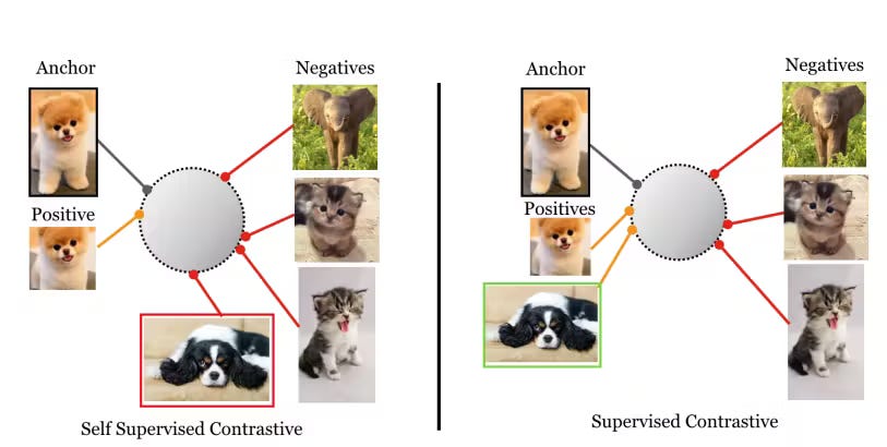
At the heart of contrastive learning lies the goal of learning data representation for which positive pairs (similar samples) are pulled closer together while negative pairs (dissimilar samples) are pushed apart. A general (more or less) mathematical formulation for the contrastive loss is for the data samples X₁ and X₂ (images, text, audio etc):

\(L(Y, X_1, X_2)) = (1 - Y)L_S(D(X_1, X_2)) + YL_D(D(X_1, X_2)), \text{ where}\)

• Y=0 indicates that the two given data points (X₁ and X₂) are similar, whereas Y=1 signifies that they are dissimilar. X

• Ls​ represents the loss function applied when the given samples are similar, while Ld​ is the loss function used when the data points are dissimilar.

• D​ denotes the measure of similarity (actually dissimilarity) between X₁ and X₂.

The measure of similarity Dw can take just the euclidian distance(aka L2) between the embedding of X₁ and X₂, computed, for example, by a neural network f parametrized with the weight vector W:

\(D(X_1, X_2) := D_W(X_1, X_2) = \|f_W(X_1) - f_W(X_2)\|_2\)

For example, contrastive loss between X₁ and X₂, can be computed in the following manner:

\(\mathcal{L}(X_1, X_2) = Y \cdot \| f_W(X_1) - f_W(X_2) \|^2 + (1 - Y) \cdot \max(0, m - \| f_W(X_1) - f_W(X_1) \|)^2 \)

where m is a margin ensuring dissimilar pairs are sufficiently far apart.

Other loss functions used with the contrastive learning are Triplet Loss and InfoNCE Loss.

Contrastive Loss Variants: Triplet Loss

Triplet Loss extends the contrastive loss by operating on triplets: an anchor sample x_a, a positive sample x_p (similar to the anchor), and a negative sample x_n (dissimilar to the anchor). The goal is to ensure the anchor-positive distance is smaller than the anchor-negative distance by at least a margin m:

\(\mathcal{L}_{\text{triplet}} = \max(0, \| f(x_a) - f(x_p) \|^2 - \| f(x_a) - f(x_n) \|^2 +m)\)

How It Works:

1. The triplet network embeds all 3 samples (x_a, x_p, x_n) into a shared space.

2. A distance metric, such as Euclidean or cosine distance, is used to compute distances between the embeddings.

3. The network learns to minimize the anchor-positive distance and maximize the anchor-negative distance.

   

Applications:

1. Face Verification and Recognition: Used in models like FaceNet for learning compact facial embeddings. For example, FaceNet maps faces into a Euclidean space where similar faces cluster together.

2. Metric Learning: Often applied in image retrieval systems to rank similar images higher in searches.

3. Speaker Verification: Helps differentiate voices in audio datasets by embedding similar voices closer together.

Challenges:

• Requires careful triplet mining to ensure training efficiency. Poorly chosen triplets can slow down convergence.

Contrastive Loss Variants: InfoNCE

InfoNCE (Information Noise-Contrastive Estimation) loss is a contrastive loss function widely used in representation learning, particularly in self-supervised learning tasks. It aims to maximize the mutual information between paired samples (e.g., anchor and positive samples) while minimizing similarity with negative samples. InfoNCE works by creating a probabilistic discrimination task where the model predicts which positive sample corresponds to an anchor among a set of negative samples. This is achieved by optimizing the following loss function:

\(\mathcal{L}_{\text{InfoNCE}} = -\frac{1}{N} \sum_{i=1}^N \log \frac{\exp\left(\frac{\text{sim}(f(\mathbf{x}_i), f(\mathbf{x}_i^+))}{\tau}\right)}{\sum_{j=1}^M \exp\left(\frac{\text{sim}(f(\mathbf{x}_i), f(\mathbf{x}_j))}{\tau}\right)}\)

• sim(f(x_i) ​,f(x_j​) represents the similarity between the embeddings x_i and x_j, often computed as a dot product or cosine similarity,

• xi+​ is the positive sample embedding corresponding to the anchor x​_i,

• τ is a positive temperature scaling parameter. τ controls the smoothness of the similarity distribution between samples. A higher temperature (τ>1) softens the similarity scores, making the model less confident in distinguishing between positive and negative pairs. Conversely, a lower temperature τ<1 sharpens the distribution, making the model more confident and potentially more sensitive to small differences in similarity. The choice of temperature allows for fine-tuning the contrastive learning process, balancing between exploration (higher τ) and exploitation (lower τ).

• N is the batch size, and M is the total number of samples (including negatives). The higher number of negative examples works better but impose higher computational costs.

  

Advantages of InfoNCE:

1. Effective Representation Learning: It excels at learning meaningful and discriminative features by maximizing mutual information between positive pairs.

2. Broad Applicability: InfoNCE can be applied across various domains like computer vision, natural language processing, and audio processing, making it highly versatile.

3. Contrastive Mechanism: The contrastive approach ensures the model focuses on relevant features by distinguishing between positive and negative samples.

Disadvantages of InfoNCE:

1. Dependence on Negative Sampling: Its effectiveness heavily relies on having a large and diverse set of negative samples, and poor sampling can significantly hurt performance.

2. Computational Cost: The need to compute similarities for all pairs, particularly with large negative sample sets, can make it computationally intensive.

Prominent Contrastive Learning Methods

1. SimCLR: Simplified Contrastive Learning of Visual Representations

Domain: Computer Vision

Key Idea: SimCLR relies on data augmentations to create positive pairs. Each image is augmented (e.g., cropping, flipping, color jittering) to generate two correlated views of the same image. All other images in the batch serve as negative samples. The network minimizes the InfoNCE loss:

\(\mathcal{L}_{i,j} = -\log \frac{\exp(\text{sim}(f(x_i), f(x_j))/\tau)}{\sum_{k=1}^{2N} \mathbf{1}_{[k \neq i]} \exp(\text{sim}(f(x_i), f(x_k))/\tau)}, \text{ where}\)

\(\text{sim}(z_i, z_j) = \frac{z_i \cdot z_j}{\|z_i\| \|z_j\|} \text{ is cosine similarity} \text{ and} f \text{ is an embedding function}\)

\(\text{ and} f(x) \text{ is a data embedding function e.g. neural network}\)

Additional Details about :

• Architecture: SimCLR uses a backbone (e.g., ResNet) to extract features and a projection head (MLP) to map these features into a space where contrastive learning is applied.

• Augmentation Strategy: Strong augmentations like random cropping and Gaussian blurring are crucial to encourage the network to learn invariances.

Impact:

• Improved performance on downstream tasks like image classification.

• Significant reductions in labeled data requirements.

Challenges:

• Requires large batch sizes to generate diverse negatives, which can be computationally expensive

  

2. MoCo: Momentum Contrast

Domain: Computer Vision

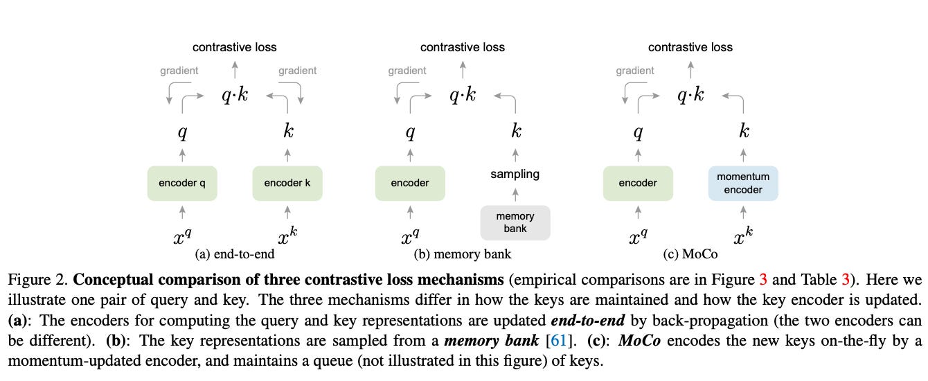
Key Idea: Momentum Contrast (MoCo) addresses the batch size limitation of SimCLR by maintaining a memory queue of negative samples. A momentum encoder generates embeddings for the negatives, ensuring consistency over time.

How It Works:

1. The data sample embeddings are computed using a query encoder.

2. The keys (negatives) are generated using a momentum encoder.

3. The memory queue stores a dynamic set of negative embeddings, which is updated as training progresses.

Loss Function: Similar to SimCLR but operates on the memory queue, reducing the reliance on large batch sizes.

Advantages:

• Scales well with smaller batch sizes due to the memory queue.

• Ensures stable training by using a slowly updated momentum encoder.

Applications:

• Widely used in video understanding tasks where long-term temporal dependencies require consistent representations.

  

3. BYOL: Bootstrap Your Own Latent

Domain: Self-Supervised Learning in Computer Vision

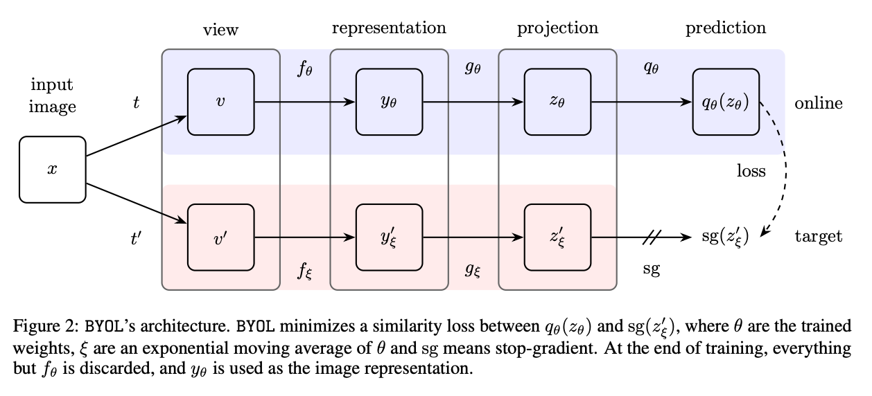
Key Idea: Unlike SimCLR and MoCo, BYOL eliminates the need for negative samples. It trains a student network to predict the output of a teacher network, which is a moving average of the student.

Loss Function: BYOL minimizes the mean squared error between the normalized embeddings of the student f(x_s) and the teacher f(x_t):

\(\mathcal{L}_{BYOL} = \| f(x_s) - f(x_t) \|^2\)

How It Works:

1. Two views of the same image are generated through augmentations.

2. The student network processes one view, while the teacher network processes the other.

3. The student learns to predict the teacher's embeddings.

Impact:

• BYOL outperforms SimCLR and MoCo in many cases.

• Its simplicity and lack of negatives make it easier to scale.

Challenges:

• Can require careful tuning of the momentum parameter for the teacher network.

  

4. CLIP: Contrastive Language-Image Pretraining

Domain: Cross-modal Learning (NLP + Vision)

Key Idea: CLIP learns joint embeddings for text and images. It contrasts matched image-text pairs against mismatched ones, using datasets of image-caption pairs.

Loss Function: A cross-modal extension of the InfoNCE loss, where each positive and negative pair consist of an image and a caption(text).

Additional Details:

• Architecture: CLIP uses separate encoders for images (e.g., Vision Transformers) and text (e.g., Transformer-based language models).

• Applications: CLIP excels in zero-shot classification, image-text retrieval, and multimodal understanding tasks

  

Contrastive Learning in Audio Processing

1. COLA: Contrastive Learning of Audio Representations

Domain: Audio Representation Learning

Key Idea: COLA adapts contrastive learning for audio data. It generates positive pairs by applying augmentations like time-stretching, pitch-shifting, and noise addition.

2. Wav2Vec

Domain: Speech Recognition

Key Idea: Wav2Vec learns latent speech representations by contrasting different segments of audio. The pre-trained embeddings are fine-tuned for tasks like ASR.

Impact:

• Robust to noise and variations in audio data.

• Reduces labeled data requirements for speech recognition

Concluding Thoughts

Contrastive learning has reshaped the way we approach self-supervised and unsupervised learning. Its mathematical foundation and adaptability across domains make it a cornerstone of modern AI. With advancements in methods like BYOL, SimCLR, and CLIP, we witnessed a paradigm shift in representation learning, reducing our reliance on labeled data while achieving state-of-the-art performance.