


A Survey on Diffusion Models for Inverse Problems
Deep Learning Paper Review: Mike's Daily Article Review - 27.01.25

Diffusion models have rapidly emerged as a powerful tool for generative modeling, capable of producing high-quality samples across diverse domains. Their success has paved the way for groundbreaking advancements in solving inverse problems, particularly in image restoration and reconstruction, where diffusion models serve as unsupervised priors.
The survey, I am going to review today, offers a comprehensive exploration of methods leveraging pre-trained diffusion models to address inverse problems without the need for additional training. The authors present a structured taxonomy that categorizes these approaches based on the specific problems they tackle and the techniques they employ.
Mathematical Framework for Inverse Problems
The paper formalizes inverse problems under the general formulation:
where A is a (possibly nonlinear) corruption operator, and controls the noise level, X is an original clean data and Y is corrupted data. Various well-known problem settings, such as denoising, inpainting, and compressed sensing, are framed within this formulation by specifying different forms of A.
2. Diffusion Processes
The authors leverage Denoising Diffusion Probabilistic Models (DDPMs) and their extensions based on stochastic differential equations (SDEs) to approach inverse problems. The forward process is described by:
where W_t is a Wiener process, X_t is data distribution at iteration(time) t. f and g are hyperparameters of the diffusion process(noise schedule). Anderson’s reverse Stochastic Differential Equations(SDE) framework is used to sample from the unknown data distribution:
This formulation enables modeling corrupted data by progressively adding noise and subsequently reversing the diffusion process for reconstruction. The core mathematical challenge is estimating the score function which is the gradient of the probability distribution p_t(x_t). The survey highlights the pivotal role of Tweedie’s formula:
Learning the conditional expectation using neural networks provides an effective way to approximate the score.
3. Taxonomy of Methods in Diffusion-Based Inverse Problem Solving
The authors of the paper provide a rich taxonomy that categorizes methods based on their mathematical approach, target problem types, and optimization techniques.
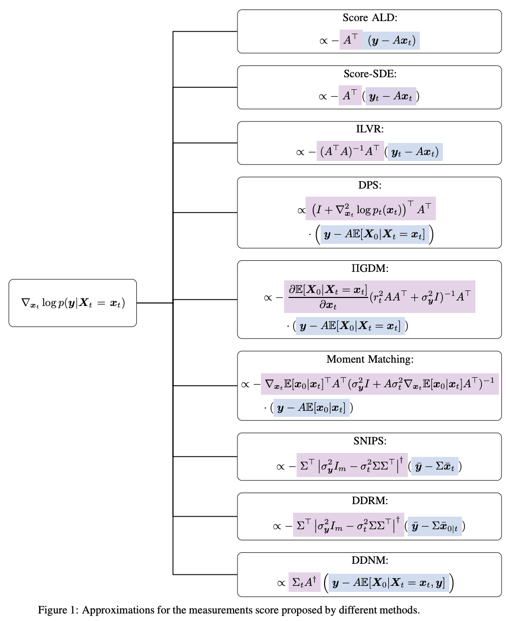
3.1 Explicit Approximations for Measurement Matching
This family focuses on approximating the measurement score term in a diffusion framework. These approximations often leverage closed-form solutions for linear inverse problems. The general form is given by:
where:
L_t represents the measurement error, typically defined as .
M_t projects the error back into the solution space; for example, in linear cases.
G_t is a re-scaling factor controlling guidance strength.
y is corrupted data
x_t is a noised version of the reconstructed original data.
Representative Methods
Score-ALD (ALD stands for Annealed Langevin Dynamics): Uses a simple approximation:
\(\nabla_{x_t} \log p(y | x_t) \approx -\frac{A^T (y - A x_t)}{\sigma_y^2 + \gamma_t^2}.\)DPS (Diffusion Posterior Sampling): Approximates the posterior using a mapping:
\(p(y | X_0 = \mathbb{E}[X_0 | X_t]) \sim \mathcal{N}(y; A \mathbb{E}[X_0 | X_t], \sigma_y^2 I),\)
leading to:\(\nabla_{x_t} \log p(y | x_t) \propto A^T (y - A \mathbb{E}[X_0 | X_t]).\)Moment Matching: Extends DPS by incorporating an anisotropic Gaussian approximation:
\(p(x_0 | x_t) \approx \mathcal{N}(\mathbb{E}[X_0 | X_t], \sigma_t^2 \nabla_{x_t} \mathbb{E}[X_0 | X_t]).\)
4.2 Variational Inference Methods
These methods approximate the true posterior distribution by introducing a tractable surrogate distribution and optimizing its parameters via variational techniques. The goal is to minimize the KL divergence between the surrogate and true posterior:
\min_{q} D_{KL}(q(x) \| p(x | y)).
Key Techniques:
RED-Diff: Proposes a novel loss combining reconstruction and score-matching objectives:
\(\mathcal{L}_{\text{RED}}(\mu) = \frac{1}{2 \sigma_y^2} \| y - A \mu \|^2 + \sum_t \lambda_t \| \epsilon_\theta(x_t) - \epsilon \|^2,\)where μ is the variational mean, and ε_θ is the denoising function learned by the diffusion model.
Blind RED-Diff: Extends RED-Diff by jointly optimizing for both the latent image and forward diffusion model parameters . This leads to a coupled variational problem:
\(\min_{q} D_{KL}(q(x, \phi) \| p(x, \phi | y)). \)where φ is a neural network extraction latent representation of data.
4.3 CSGM-Type Methods (Conditional Score Generative Models)
These approaches optimize directly over a latent space using backpropagation. The fundamental idea is to iteratively adjust initial noise vectors to satisfy measurement constraints.
Key Techniques
Backprop through a deterministic diffusion sampler.
Latent space optimization to enforce fidelity to the observed measurements.
4.4 Asymptotically Exact Methods
These methods rely on sampling from the true posterior distribution using advanced Markov Chain Monte Carlo (MCMC) techniques.
Key Techniques
Particle Propagation: Sequential Monte Carlo (SMC) methods propagate multiple particles through distributions to approximate the posterior.
Twisted Sampling: Methods like the Twisted Diffusion Sampler (TDS) use geometry-aware updates to enhance convergence rates.
4.5 Optimization Techniques
The methods further vary by the optimization strategies employed:
Gradient-based techniques: Utilize derivatives to enforce measurement consistency.
Projection-based techniques: Project samples onto feasible subspaces.
Sampling techniques: Use probabilistic approaches like Langevin Dynamics for particle updates.
This survey elegantly brings together advanced mathematical tools, providing a solid foundation for researchers aiming to solve inverse problems using diffusion processes. The integration of stochastic calculus, Bayesian inference, and optimization techniques makes it a crucial reference point for pushing the boundaries of inverse problem-solving.
https://arxiv.org/pdf/2410.00083