
A Route to Large Language Models: A Historical Review
Joint work with Hay Hoffman


Introduction
This article explores one of the most fascinating applications of Transformer architecture: Large Language Models (LLMs). While these models have been around in Machine Learning for some time, their remarkable effectiveness across so many tasks raises fundamental questions about how they work, how best to train them, and what makes them so powerful.
The development happened gradually, but at a certain point, these models created a paradigm shift in Natural Language Processing. Before LLMs, language models were typically designed for specific tasks like part-of-speech tagging, summarization, or question answering. LLMs changed the game by offering a "mega-model" capable of handling a wide variety of tasks successfully.

Figure 1: Transformer architecture
The purpose of this article is to present an overview of LLMs historical development, the theoretical infrastructure underlying them, and the methodologies used for training them. It's important to emphasize that the process of training a language model is a complex challenge, involving tasks such as: creating and cleaning quality datasets, implementing advanced training techniques and more. The article's goal is not to provide an exhaustive review of all existing methods, but rather to give the reader a deep understanding of the essential building blocks in training models of this type.
Important note: A language model is an idea, while Transformer-based models are one way to implement it. In practice, language models are not bound to implementation through Transformers, and can be implemented using models with different architectures such as RWKV or Mamba.
Additional note: We refer to any model whose purpose is to perform language-related tasks using the term Language Model even when we are not referring to a specific architecture or task. In contrast, when we mention the term “Large Language Model” in the text, we are referring to a language model that has been trained on an enormous amount of text and is capable of performing a wide range of language tasks without additional dedicated training.
Before we begin the discussion, let's define the terms we'll be using:
Dictionary: A finite set of words, where each word has a semantic meaning in the language. The dictionary contains the words that the model can recognize and process, where each word in the dictionary is represented by a unique numerical value that serves as its ordinal number in it.
Text: A sequence of words (which can include symbols, numbers, punctuation marks, and letters/words from different languages). The text is not limited in length (but is finite) and can only be composed of words that exist in the dictionary.
Language: The set of all possible texts. Theoretically, this set is infinite, since one can take any text, add more words to it, and thereby create a new text.
Dataset: A collection of texts sampled from the language. The difference between it and the language is that language is not limited in the number of examples or their length, while the dataset is. We consider the dataset as a sample of natural language; the larger and more diverse it is, the better it will represent the language as an approximation.
What is language modeling?
Why is language modeling such a challenging task?
Have you ever wondered how young children learn language? How can a toddler look at an orange fruit with a green leaf and simply say "orange"? This question points to a fundamental mystery: how do specific words become connected to the ideas they represent? Or put another way, how do we teach semantics?
This is the essence of language: our ability to describe ideas through a limited set of symbols that both speaker and listener understand. We're exploring this question because it directly relates to the first chapter's purpose: to examine how we can "explain" natural language to a statistical model and effectively represent it.
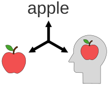
Figure 2: A central topic in semantics concerns the relation between language, world, and mental concepts.
But what does "explain" really mean when talking about language models? This leads us to a deeper look at how humans understand and process language.
Human language understanding is complex and deeply rooted in our physical experience of the world. Words and concepts in our minds connect to sensory experiences, daily interactions, and our physical existence. When a child learns the word "orange," they're not just hearing a sound or seeing a symbol – they're feeling its texture, tasting its flavor, and smelling its distinctive scent. This is true multi-sensory learning, anchored in real-world experience.
In contrast, language models are machines without physical embodiment. They operate in a world of symbols and patterns, without any sensory foundation or the context of real life. When we "teach" a language model, we are essentially feeding it abstract linguistic patterns, from which it can generalize and identify linguistic structures. This is the fundamental difference - while human understanding is based on tangible experience, the model's "understanding" is limited solely to data processing and identifying correlations.
These claims are exemplified by philosophical thought experiments such as Searle's Chinese Room. This experiment argues that even if a machine passes the Turing test (meaning one cannot distinguish whether they're talking to a human or model), this doesn't prove genuine understanding, since such a machine can perform predefined manipulations on symbols just as a one who doesn't speak Chinese could answer questions in Chinese using a predefined set of rules for each input.
Much like Searle's thought experiment suggests, today's models can appear to understand natural language (like in translation tasks requiring context) without connecting to sensory experience or physical existence. While their ability to handle complex pattern-based tasks highlights their potential, it also reveals limitations in truly understanding language and meaning. This fundamental limitation explains why models struggle with concepts requiring grounded experience, such as physical relationships, temporal sequences, and intuitive world knowledge.
How is language represented quantitatively?
The previous chapter examined the philosophical aspects of language understanding in computational models. While the basic assumption is that current language models can process and understand language to some degree, yet the exact meaning of this "understanding" remains an open question. This chapter will focus on the practical aspect of quantitative language representation, seeking to answer: how can words and their relationships be represented efficiently for these language models to process?
A persistent challenge in computational linguistics has been: how can we mathematically represent language in ways machines can process? To illustrate why this is difficult, consider how humans naturally understand language. When we hear "The cat walks in the garden" and "The dog walks in the house," we instinctively categorize words by function – "the" identifies nouns, "cat" and "dog" are actors, "walks" describes the action, "in" indicates position, and "garden" and "house" are locations. These intuitive groupings correspond to formal grammatical categories:
[determiners ("the"), subjects ("cat," "dog"), predicates ("walks"), prepositions ("in"), and location objects ("garden," "house").]
While this categorization happens effortlessly in our minds, thanks to our innate understanding of language and the world, teaching computers to make these same connections has proven to be remarkably challenging using deterministic methods.
What's even more fascinating is how this intuitive understanding extends to new sentences. Consider "The lion roams in the cage" – even without formal grammar training, most people can instantly recognize that "lion" serves the same role as "cat" and "dog," and "cage" functions like "garden" and "house" in our previous examples. This ability to recognize patterns and relationships between words doesn't rely on knowing technical terms like "determiner" or "preposition" – it stems from our fundamental understanding of how language and the world work together.
While humans instinctively understand language patterns, machines must rely on rigid linguistic frameworks to process text. For example, creating a system that can identify parts of speech requires building an intricate network of language rules - from basic grammar to word meanings - and maintaining extensive word-function dictionaries. Such a system would methodically analyse each word's context, identify its grammatical role, and decode sentence structure. It will do this by consulting its dictionary for possible word functions, then applying grammatical rules to resolve uncertainties and determine the most appropriate interpretation.
Rule-based language processing faces two critical constraints that highlight the gap between machine and human capabilities. The first is their inability to handle novel situations not covered by their predefined rules and dictionaries. The second is the inherent challenge of encoding the full spectrum of natural language into a limited ruleset. This limitation becomes particularly evident when we consider Zipf's law, which demonstrates how language naturally organizes itself: a small set of words dominate usage frequency, while countless rare words form an extensive tail of occasional occurrences.
A more effective solution emerges through Machine Learning, which excels at recognizing patterns rather than following explicit rules. This approach learns from data and generalizes to new situations - particularly useful for semantic tasks like the part-of-speech tagging discussed earlier. But this raises an interesting question: if we can't explicitly program linguistic rules, how do we enable a language model to understand them? The key lies in implicit learning - allowing the model, functioning as a statistical processor, to discover language patterns on its own. Rather than being programmed with specific word properties, the model learns the statistical relationships between words in different contexts. For example, it naturally discovers that 'apple' frequently appears alongside words like 'tasty,' 'red,' or 'tree,' and learns how context influences word meaning.
Although machine learning can implicitly learn word relationships and contexts, implementing this capability requires addressing a critical challenge: converting linguistic input into numerical form. The standard approach of assigning dictionary indices to words undermines the very semantic patterns the model needs to learn. For instance, if 'orange' becomes index 17 and 'apple' index 233, their numerical difference of 216 carries none of the semantic relationship we'd want the model to understand. This presents a paradox: while we want the model to learn rich semantic relationships, our basic numerical representation does not model these relationships correctly. The arbitrary nature of dictionary indices contradicts a core principle of machine learning: that similar meanings should have similar numerical representations. This mismatch impairs the model's ability to learn meaningful language patterns.
One solution to the challenge of NLP is to learn continuous representations of words within a shared vector space. Each dimension within this space corresponds to a distinct feature, and its value is derived from both the word's semantic meaning and its co-occurrence patterns with other words (based on examples in the dataset). Consider the task of identifying parts of speech within a sentence. To accomplish this, we can create a dataset of labeled examples, where the input consists of natural language sentences, and the desired output is the accurate tagging of each word according to its syntactic role. During the model training process, we update both the model's weights and the vectors representing words in the shared space. However, this approach presents several challenges. One issue is the interdependence between finding representation vectors and training the network for the specific task. The model learns vector representations that are specifically tailored to the task it's being trained on, which limits the ability of the vectors to generalize to other tasks.
The second problem with task-specific modeling lies in the statistical distribution characteristics of the data. The probability density function of a task-specific dataset tends to concentrate in narrow regions of the general semantic distribution space, whereas optimal language representation requires the dataset to represent it comprehensively, not just focus on certain aspects. Since creating a high-quality dataset for tagging tasks requires substantial resources, most datasets used for these tasks are relatively small. The optimal solution to this challenge lies in using massive unlabeled datasets (essentially, all textual information available on the internet) while implementing unsupervised learning or self-supervised learning methods. This approach allows the model to acquire a rich and accurate semantic representation of language, while overcoming the bias limitations and data scope constraints inherent in traditional supervised learning methods.
How do we estimate the joint probability of words?
At this point, we face a fundamental methodological challenge - in the absence of a defined learning task, what is the optimal objective function for the learning process? The answer is estimating the joint probability of a sequence of words appearing together. Under this assumption, we treat the model as a statistical machine that estimates a function p(X) representing the joint probability of appearing of a word sequence X = x_1, x_2 , . . .,x_n. Under this paradigm, the model is represented as function q(X) that approximates p(X), where is a set of parameters (if our model is a neural network for example, is its set of weights). An important point to understand is that p(X) is not explicitly known to us and we will need to find a way to approximate q to p through learning.
The traditional approach to learning a probability function is through distance functions that measure the difference between two distributions: the "true" distribution, represented by the dataset, and the model's learned approximation of it. In our case, we'll use the Kullback-Leibler (KL) divergence, which allows us to quantify how far q(X) is from p(X), given the "true" probability p(X) and the learned probability q(X). However, it is important to note that utilization of the KL distance necessitates knowledge of the true p(X). However, it is important to note that using the KL divergence requires knowledge of the true p(X). Specifically, it requires knowledge of the probability of sampling any given text segment within the dataset.
One way to estimate probability in a linguistic space (or any discrete space) is by calculating relative frequency. This involves finding the ratio between the number of times a specific word sequence appears and the total number of word sequences of the same length in the data corpus.. For example, let's consider a dataset with two sentences: "Little Jonathan went to kindergarten" and "Where did little Johnny go?" The relative frequency of a word pair, or bigram, like "little Johnny" is determined by counting all bigrams in a dataset and then counting the occurrences of the specific pair. In this instance, the bigram "little Johnny" appears twice out of six total bigrams, resulting in a relative frequency of 1/3. However, computing the entire probability space (relative frequency for every possible n-gram) is impractical, particularly for massive datasets containing tens of trillions of words, which are commonly used to train LLMs today.
We then need to search within the dataset for all occurrences of each combination we found. While there are optimization methods that can be applied during the search process, it remains computationally impractical, and this is just for texts of six words or fewer.
Beyond the computational challenge, a fundamental question arises: Is counting relative frequencies of words in text really sufficient to represent the full semantic meaning of the words within it? Research in computational linguistics presents a complex picture.
On one hand, foundational work in linguistics such as [2] introduced the idea that words appearing in similar contexts tend to carry similar meanings, followed by researches in LSA (Latent Semantic Analysis) during the 1990s, such as paper [3], that demonstrated how semantic relationships like synonyms or words with multiple meanings (such as "bat" which can mean either a flying mammal or a sports equipment) could be identified across different documents through frequency analysis. On the other hand, later studies, such as [4,5], revealed significant limitations in word representations based solely on frequency counting - they showed that this approach might miss important nuances in word meanings.
It is crucial to acknowledge that no existing research has fully modeled the probability p(X) through frequency analysis in the manner described above. Thus, the question of whether these methods can accurately represent the semantic complexity of natural language remains unanswered. Our view is that such modeling, no matter how good, would not be sufficient to fully model p(X), because language is a dynamic and changing structure, and new texts that never appeared in the modeling set can be created constantly. Additionally, counting frequencies of word sequences indicates relationships between words but does not model their meaning.
So what's the solution? Maximizing the likelihood function for dataset D given model q_θ(X).
What is the likelihood function?
The likelihood function, used in training language models, can be explained by starting with a general example to illustrate how it works. Imagine a detective trying to solve a complicated case. They have fixed, unchanging evidence and are considering several theories about what might have happened. Given that one of these theories must be correct, how will the detective know which one? They need to find some tool that measures how well each theory explains the evidence, and the theory that gets the highest score will be the correct one. This is what the likelihood function does - the fixed evidence is our dataset, and the theories being considered are models that model different probability functions.
In general, the likelihood function is described as follows:
Given a model f that is parameterized by a set of weights (a specific theory), the likelihood function describes the probability of sampling dataset D using it (how well the theory explains the evidence). The model is a mathematical function f of some form (architecture in the case of deep models) defined by a set of parameters (for example, model weights) over our data space D (such as text segments).
Let's denote f(X, θ) = q_θ(X), and consequently, the likelihood function takes the following form:
However, what are the different theories we can examine here? In other words, what are the different q_θ(X) functions that we're considering against each other? As we mentioned, the model and set of weights define the function q_θ(X), so we need to measure how well q, defined by the set of parameters , approximates the true p(X). What defines the different models in this case is the set of parameters for a fixed architecture, meaning we can view the model at different training stages as a set of different models q_1, q_2, . . . , q_n where each set of weights defines a different model. The goal of learning is to find the optimal set of weights that predicts the dataset maximally by minimizing the cost function.
How do we actually do this?
Our goal is to maximize the likelihood function for a given dataset D. Therefor, we aim to maximize the probability of sampling the entire dataset D with function(model) q_θ. The mathematical expression of this goal is given by the following equation:
Maximizing this expression could be numerically unstable since it contains a product of an enormous number of values smaller than 1 (q_θ(X) is a value between 0 and 1 for each X). To overcome this, we use the logarithm function to eliminate the product and convert it into a sum in the following way:
Since X is a sequence of words x_1, x_2, ... , x_n, we use the chain rule of probability in the following way:
where nX denotes the number of tokens in example X and x_{1 : i-1} = x_1, x_2, ... , x_{i-1}. Here we assume that the next word(token) distribution is fully determined by the preceding words.
We substitute the expression for q_θ(X) into the likelihood function of dataset D, and get:
Due to historical conventions in machine learning, we work with the Negative Log Likelihood (NLL) rather than directly maximizing the log-likelihood function. By taking the negative logarithm of the likelihood function, we convert our maximization problem into a minimization problem - minimizing the NLL is equivalent to maximizing the original likelihood. This transforms our function into:
Given the massive size of our dataset, computing NLL gradients over the entire dataset for each weight update would be computationally intractable. Instead, we use Stochastic Gradient Descent (SGD), which samples mini-batches of data and assumes their NLL values approximate the average NLL of the full dataset. This yields the following estimator for the dataset likelihood function E[D] based on mini-batch B:
where 1/B normalizes by the mini-batch size.
Alternative Interpretation of NLL
The NLL function can be interpreted through the KL divergence between our model's output distribution and the true text distribution. Since we don't have access to the true text distribution p, we approximate it using dataset samples. Instead of working with unknown distributions - the sample distribution pX and its conditional word probabilities given previous context x_{1 : i-1} - we use a degenerate conditional distribution concentrated on the actual words x_i for x_i, ∀ i ∊ [1, n_x].
Therefore, it follows that:
When we look at p(X), which we don't know from our dataset, and all the conditional probabilities that come from it, we mean that even when we know what words in x_{1 : i-1} series, we still don't know exactly how likely each possible next word x_i is. These probabilities are spread out across many different words in our dictionary.
For example, in the sentence "Kids aged 3 to 5 usually like", the next word could be [chocolate, fruit, to play, other kids,..., toys], where each possible word has its own conditional probability value based on the dataset.
Since we don't know this probability distribution, we use the only conditional distribution we do know - the actual next word in our example that gets all the probability weight (1), while all other words in the dictionary get 0. We believe that with a sufficiently diverse dataset, the model will learn to approximate the true conditional distribution of the dataset through these various examples.
For a given example in the mini-batch, we can apply Bayes' rule to p(X) and express it through conditional distributions (degenerate ones) in exactly the same way we do for the model q_θ(X).
Since we're now dealing with two conditional distributions
we can see that the NLL expression equals the cross-entropy between these two distributions:
Since
and 0 for all other words in the dictionary, the cross-entropy actually equals the logarithmic likelihood function:
How does the cross-entropy expression relate to KL divergence in optimization problems over qθ (general case)?
It's known that the following relationship holds between cross-entropy and KL divergence for any two distributions p and q_θ :
In other words, the cross-entropy equals the difference between the KL divergence of q_θ and p and the entropy of p. Since H(p(X)) (the entropy of distribution p) is constant with respect to the optimization parameters θ, we can ignore it when optimizing for q_θ. Therefore, any q_θ that minimizes H(p, q_θ) necessarily minimizes D_KL(p||q_θ).
Conclusion
In this article we reviewed the foundations of natural language modeling and demonstrated why purely rule-based linguistic modeling is impractical for highly complex text. We examined various unsupervised machine learning methods for understanding word semantics and presented the theoretical basis for natural language modeling: next-word prediction using a likelihood function. We focused on this method as it forms the cornerstone of training LLMs.
In the next chapter, we'll explore the field's evolution, from static word embeddings through context-dependent dynamic representations (contextualized embeddings), to the advanced methods that enable the impressive capabilities we see in today's LLMs.
Bibliography
1. Vaswani A et al. Attention is all you need, 2017, http://arxiv.org/abs/1706.03762
2. Harris ZS. Distributional Structure. 1954, https://books.google.com/books/about/Distributional_Structure.html?hl=&id=ycMmcgAACAAJ
3. Landauer T.K., Dumais S.T., A solution to Plato’s problem: The latent semantic analysis theory of acquisition, induction, and representation of knowledge, Psychol. Rev. 1997;104: 211–240. doi:10.1037/0033-295x.104.2.211
4. Baroni M, Dinu G, Kruszewski G., Don’t count, predict! A systematic comparison of context-counting vs. context-predicting semantic vectors. In: Toutanova K, Wu H, editors. Proceedings of the 52nd Annual Meeting of the Association for Computational Linguistics (Volume 1: Long Papers). Association for Computational Linguistics; 2014. pp. 238–247. doi:10.3115/v1/P14-1023
5. Faruqui M, Tsvetkov Y, Rastogi P, Dyer C. Problems with evaluation of word embeddings using word similarity tasks, 2016, http://arxiv.org/abs/1605.02276
Want to connect with us? -> Find us on LinkedIn: Hay and Michael
Hay is an AI engineer focused on developing intelligent autonomous agents using LLMs. He holds a Master's degree in Computer Science from Ariel University.
Mike is an AI expert with a PhD in Mathematics, leading AI development at a stealth company. As a science content creator and lecturer, he has reviewed over 400 papers in deep learning and hosted more than 40 podcasts, building a following of over 50,000 on LinkedIn. Mike dedicates his time to making complex AI knowledge accessible to the professional community.
 | A guest post by
|